记录一次kaggle比赛，这次比赛的场景主要是Jane Street日内高频交易，是短线模型，使用夏普率衡量模型效果，但是提供的数据并非原始数据，不清楚feature含义。

1. Overview

1.1 Description

In a perfectly efficient market, buyers and sellers would have all the agency and information needed to make rational trading decisions. As a result, products would always remain at their “fair values” and never be undervalued or overpriced. However, financial markets are not perfectly efficient in the real world.

Even if a strategy is profitable now, it may not be in the future, and market volatility makes it impossible to predict the profitability of any given trade with certainty.

1.2 Evaluation

• Utility score

  Each row in the test set represents a trading opportunity for which you will be predicting an action value, 1 to make the trade and 0 to pass on it. Each trade j has an associated weight and resp, which represents a return.

$$
p_i = \sum_j(weight_{ij} resp_{ij} action_{ij}),
$$

$$
t = \frac{\sum p_i }{\sqrt{\sum p_i^2}} * \sqrt{\frac{250}{|i|}},
$$
where |i| is the number of unique dates in the test set. The utility is then defined as:
$$
u = min(max(t,0), 6) \sum p_i.
$$

https://www.kaggle.com/renataghisloti/understanding-the-utility-score-function

• _Pi_

  Each row or trading opportunity can be chosen (action == 1) or not (action == 0).

  The variable _pi_ is a indicator for each day _i_, showing how much return we got for that day.

  Since we want to maximize u, we also want to maximize _pi_. To do that, we have to select the least amount of negative resp values as possible (since this is the only negative value in my equation and only value that would make the total sum of p going down) and maximize the positive number of positive resp transactions we select.

• t

  _t_ is larger when the return for each day is better distributed and has lower variation. It is better to have returns uniformly divided among days than have all of your returns concentrated in just one day. It reminds me a little of a _L1_ over _L2_ situation, where the _L2_ norm penalizes outliers more than _L1_.

Basically, we want to select uniformly distributed distributed returns over days, maximizing our return but giving a penalty on choosing too many dates.

• t is simply the annualized sharpe ratio assuming that there are 250 trading days in a year, an important risk adjusted performance measure in investing. If sharpe ratio is negative, utility is zero. A sharpe ratio higher than 6 is very unlikely, so it is capped at 6. The utility function overall try to maximize the product of sharpe ratio and total return.

2. Implementing.

https://www.kaggle.com/vivekanandverma/eda-xgboost-hyperparameter-tuning

https://www.kaggle.com/wongguoxuan/eda-pca-xgboost-classifier-for-beginners

https://www.kaggle.com/smilewithme/jane-street-eda-of-day-0-and-feature-importance/edit

2.0 Preprocessing

2.1. EDA

Market Basics: Financial market is a dynamic world where investors, speculators, traders, hedgers understand the market by different strategies and use the opportunities to make profit. They may use fundamental, technical analysis, sentimental analysis,etc. to place their bet. As data is growing, many professionals use data to understand and analyze previous trends and predict the future prices to book profit.

Competition Description: The dataset provided contains set of features, feature_{0…129},representing real stock market data. Each row in the dataset represents a trading opportunity, for which we will be predicting an action value: 1 to make the trade and 0 to pass on it.

Each trade has an associated weight and resp, which together represents a return on the trade. In the training set, train.csv, you are provided a resp value, as well as several other resp_{1,2,3,4} values that represent returns over different time horizons.

In Test set we don’t have resp value, and other resp_{1,2,3,4} data, so we have to use only feature_{0…129} to make prediction.

Trades with weight = 0 were intentionally included in the dataset for completeness, although such trades will not contribute towards the scoring evaluation. So we will ignore it.

2.2 Using XGBoost Algorithm

XGBoost?

it is contents of ensemble learning.

https://www.youtube.com/watch?v=VHky3d_qZ_E

https://www.youtube.com/watch?v=1OEeguDBsLU&list=PL23__qkpFtnPHVbPnOm-9Br6119NMkEDE&index=4

https://www.youtube.com/watch?v=4Jz4_IOgS4c

https://www.youtube.com/watch?v=VkaZXGknN3g&feature=youtu.be

https://bkshin.tistory.com/entry/%EB%A8%B8%EC%8B%A0%EB%9F%AC%EB%8B%9D-15-Gradient-Boost

2.2.1 Ensemble learning

x - dataset, y - error rate, each color is algorithm.

• No Free Lunch Theorem.
  • any classification method cannot be superior or inferior overall

Ensemble means harmony or unity.

When we predict the value of a data, we use one model. But if we learn several models in harmony and use their predictions, we’ll get a more accurate estimate.

Ensemble learning is a machine learning technique that combines multiple decision trees to perform better than a single decision tree. The key to ensemble learning is to combine several weak classifiers to create a Strong Classifier. This improves the accuracy of the model.

2.2.1.1 Bagging

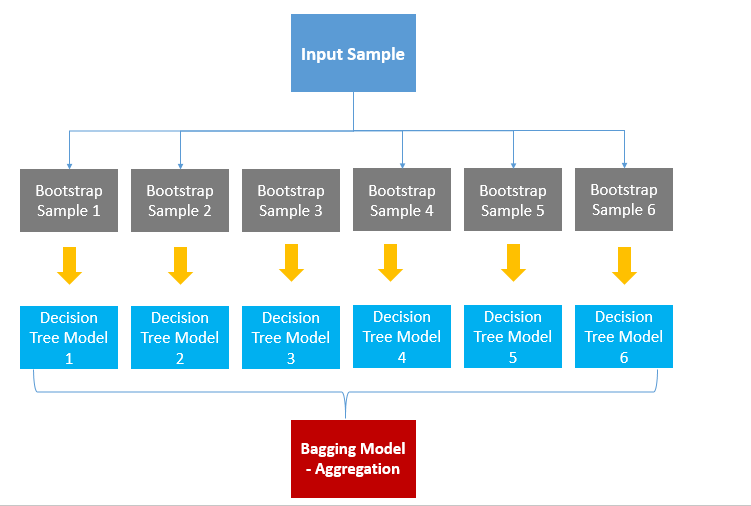
Bagging is Bootstrap Aggregation. Bagging is a method of aggregating results by taking samples multiple times (Bootstrap) each model.

First, bootstrap from the data. (Restore random sampling) Examine the bootstrap data to learn the model. It aggregates the results of the learned model to obtain the final result value.

Categorical data aggregates results in Voting, and Continuous data is averaged.

When it’s categorical data, voting means that the highest number of values predicted by the overall model is chosen as the final prediction. Let’s say there are six crystal tree models. If you predicted four as A, and two as B, four models will predict A as the final result by voting.

Aggregating by means literally means that each decision tree model averages the predicted values to determine the predicted values of the final bagging model.

Bagging is a simple yet powerful method. Random Forest is representative model of using bagging.

2.2.1.2 Boosting

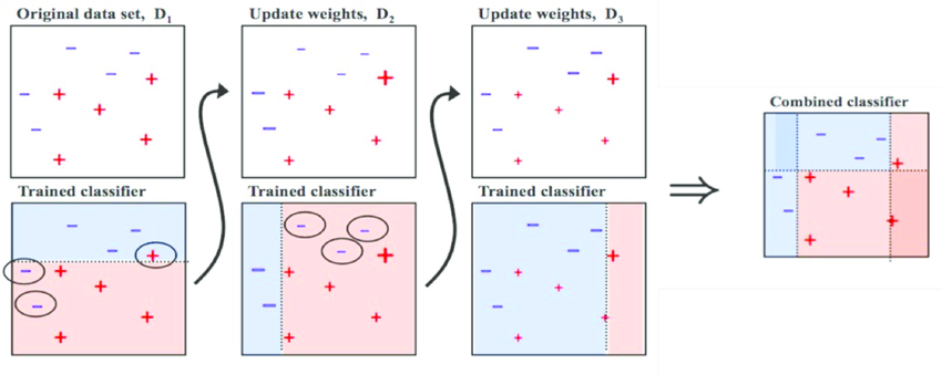
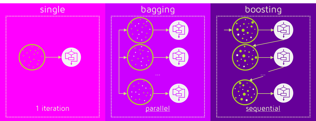
Boosting is a method of making weak classifiers into strong classifiers using weights. The Bagging predicts results independently of the Deicison Tree1 and Decision Tree2. This is how multiple independent decision trees predict the values, and then aggregate the resulting values to predict the final outcome.

Boosting, however, takes place between models. When the first model predicts, the data is weighted according to its prediction results, and the weights given affect the next model. Repeat the steps for creating new classification rules by focusing on misclassified data.

2.2.2 Different of Bagging and Boosting

Bagging is learned in parallel, while boosting is learned sequentially. After learning once, weights are given according to the results. Such weights affect the prediction of the results of the following models.

High weights are given for incorrect answers and low weights for correct answers. This allows you to focus more on the wrong answers in order to get them right.

Boosting has fewer errors compared to bagging. That is, performance is good performance. However, the speed is slow and there is a possibility of over fitting. So, which one should you choose between bagging or boosting when you actually use it? It depends on the situation. If the low performance of the individual decision tree is a problem, boosting is a good idea, or over-fitting problem bagging is a good idea.

2.2 XGBoost : A scalable Tree Boosting System(eXtreme Gradient Boosting)

https://xgboost.readthedocs.io/en/latest/

https://towardsdatascience.com/https-medium-com-vishalmorde-xgboost-algorithm-long-she-may-rein-edd9f99be63d

Optimized Gradient Boosting algorithm through parallel processing, tree-pruning, handling missing values and regularization to avoid over-fitting/bias

XGBoost = GBM + Regularization

Red part is Regularization term.

T : weak learner(node)

w : node score

Therefore, it can be seen that the regularization term of XGboost prevents overfitting by giving penalty to loss as the tree complexity increases.

2.2.1 Split finding Algorithm

• Basing exact greedy algorithm

  • Pros: Always find the optimal split point because it enumerates over all possible splitting points greedily
  • Cons:
    • Impossible to efficiently do so when the data does not fit entirely into memory
    • Cannot be done under a distributed setting

• Approximate algorithm

  • Example
    • Assume that the value is sorted in an ascending order
    • Divide the dataset into 10 buckets
    • Global variant(Per tree) vs Local variant(per split)

2.2.2 Sparsity-Aware Split Finding

• In many real-world Problems, it is quite common for the input x to be sparse
  • presence of missing values in the data
  • frequent zero entries in the statistics
  • artifacts of feature engineering such as one-hot encoding
• Solution : Set the default direction that is learned from the data

2.2.3 System Design for Efficient Computing

• The most time-consuming part of tree learning
  • to get the data into sorted order
• XGBoost propose to store the data in in-memory units called block
  • Data in each block is stored in the compressed column(CSC) format, with each column sorted by the corresponding feature value
  • This input data layout only needs to be computed once before training and can be reused in later iterations.
• Cache-aware access
  • For the exact greedy algorithm, we can alleviate the problem by a cache-aware prefetching algorithm
  • For approximate algorithms, we solve the problem by choosing a correct block size
• Out-of-core computing
  • Besides processors and memory, it is important to utilize disk space to handle data that does not fit into main memory
  • To enable out-of-core computation, the data is divided into multiple blocks and store each block on disk
  • To enable out-of-core computation, we divide the data into multiple blocks and store each block on disk
  • It is important to reduce the overhead and increase the throughout of disk IO
• Block Compression
  • The block is compressed by columns and decompressed on the fly by an independent thread when loading into main memory
  • This helps to trade some of the computation in decompression with the disk reading cost
• Block Sharding
  • A pre-fetcher thread is assigned to each disk and fetches the data into an in-memory buffer
  • The training thread then alternatively reads the data from each buffer.
  • This helps to increase the throughput of disk reading when multiple disks are available.

1
2

import numpy as np
import pandas as pd

1

train = pd.read_csv('/kaggle/input/jane-street-market-prediction/train.csv')

1
2
3
4
5
6
7
8
9
10
11
12
13
14
15
16
17
18
19
20
21
22
23
24
25
26
27
28
29
30
31
32
33
34
35
36

def reduce_memory_usage(df):
    
    start_memory = df.memory_usage().sum() / 1024**2
    print(f"Memory usage of dataframe is {start_memory} MB")
    
    for col in df.columns:
        col_type = df[col].dtype
        
        if col_type != 'object':
            c_min = df[col].min()
            c_max = df[col].max()
            
            if str(col_type)[:3] == 'int':
                if c_min > np.iinfo(np.int8).min and c_max < np.iinfo(np.int8).max:
                    df[col] = df[col].astype(np.int8)
                elif c_min > np.iinfo(np.int16).min and c_max < np.iinfo(np.int16).max:
                    df[col] = df[col].astype(np.int16)
                elif c_min > np.iinfo(np.int32).min and c_max < np.iinfo(np.int32).max:
                    df[col] = df[col].astype(np.int32)
                elif c_min > np.iinfo(np.int64).min and c_max < np.iinfo(np.int64).max:
                    df[col] = df[col].astype(np.int64)
            
            else:
                if c_min > np.finfo(np.float16).min and c_max < np.finfo(np.float16).max:
                    df[col] = df[col].astype(np.float16)
                elif c_min > np.finfo(np.float32).min and c_max < np.finfo(np.float32).max:
                    df[col] = df[col].astype(np.float32)
                else:
                    pass
        else:
            df[col] = df[col].astype('category')
    
    end_memory = df.memory_usage().sum() / 1024**2
    print(f"Memory usage of dataframe after reduction {end_memory} MB")
    print(f"Reduced by {100 * (start_memory - end_memory) / start_memory} % ")
    return df

Importing dataset

1

train = reduce_memory_usage(train)

1) import library

1
2
3
4
5
6
7
8
9
10
11
12
13
14
15
16
17
18
19
20
21
22
23
24
25
26

# This Python 3 environment comes with many helpful analytics libraries installed
# It is defined by the kaggle/python Docker image: https://github.com/kaggle/docker-python
# For example, here's several helpful packages to load

#import numpy as np # linear algebra
#import pandas as pd # data processing, CSV file I/O (e.g. pd.read_csv)
import matplotlib.pyplot as plt
import seaborn as sns
import sklearn
from sklearn.model_selection import train_test_split
from sklearn.preprocessing import StandardScaler
from sklearn.decomposition import PCA
import xgboost as xgb
import optuna
import warnings
warnings.filterwarnings("ignore")
# Input data files are available in the read-only "../input/" directory
# For example, running this (by clicking run or pressing Shift+Enter) will list all files under the input directory

import os
for dirname, _, filenames in os.walk('/kaggle/input'):
    for filename in filenames:
        print(os.path.join(dirname, filename))

# You can write up to 20GB to the current directory (/kaggle/working/) that gets preserved as output when you create a version using "Save & Run All" 
# You can also write temporary files to /kaggle/temp/, but they won't be saved outside of the current session

2) load and clean dataset

Cleaning data

1
2
3
4
5
6
7
8
9
10
11
12
13
14
15
16
17
18
19
20
21
22
23
24
25
26

# This Python 3 environment comes with many helpful analytics libraries installed
# It is defined by the kaggle/python Docker image: https://github.com/kaggle/docker-python
# For example, here's several helpful packages to load

#import numpy as np # linear algebra
#import pandas as pd # data processing, CSV file I/O (e.g. pd.read_csv)
import matplotlib.pyplot as plt
import seaborn as sns
import sklearn
from sklearn.model_selection import train_test_split
from sklearn.preprocessing import StandardScaler
from sklearn.decomposition import PCA
import xgboost as xgb
import optuna
import warnings
warnings.filterwarnings("ignore")
# Input data files are available in the read-only "../input/" directory
# For example, running this (by clicking run or pressing Shift+Enter) will list all files under the input directory

import os
for dirname, _, filenames in os.walk('/kaggle/input'):
    for filename in filenames:
        print(os.path.join(dirname, filename))

# You can write up to 20GB to the current directory (/kaggle/working/) that gets preserved as output when you create a version using "Save & Run All" 
# You can also write temporary files to /kaggle/temp/, but they won't be saved outside of the current session